Imaginary-Time Time-Dependent Density Functional Theory

Jun 20, 2019 | 14 min read | technical

Density functional theory is an approach to the electronic many-body problem in quantum mechanics used widely in in industry and academia. It is often used for calculating the properties of molecules and materials through direct simulations of their molecular and crystalline structures. While most quantum mechanical problems are solved using the Schrödinger equation, even having two quantum particles in a system can make solving the Schrödinger equation a difficult task. For example, while the Schrödinger equation for hydrogen with its single electron has a solution that is easily written down, for helium, with its mere two electrons, a closed-form solution still has not been found! Of course, approximate numerical solutions can be computed, but for molecules with their hundreds to tens of thousands of electrons, even this approach becomes impossible.

Density Functional Theory

This is where density functional theory, commonly referred to as DFT, comes into play. For a system with $N$ electrons, instead of using the many-body wavefunction that depends on $3N$ coordinates as the fundamental mathematical object, it uses the electronic density, depending only on the three coordinates of space, a substantially simpler function for humans and computers alike. Remarkably, despite appearing like a simplifying approximation, DFT is formally exact and is an equivalent view of the many-body quantum theory.

Time-Dependent Density Functional Theory

Just like in Newtonian physics where you can have static and dynamic systems, in quantum mechanics we can consider time-independent and time-dependent systems. Time-Dependent Density Functional Theory, TDDFT, applies the ideas of DFT to systems which evolve in time, due to the movement of atoms or the presence of varying electric and magnetic fields. TDDFT is commonly used in calculations of optical excitations, electronic transport, spectroscopy, electron-phonon coupling and more, since it can describe how quantum systems change as time passes.

A vacancy exciton (probably?) in a sheet of molybdenum disulfide at 300 Kelvin. Nothing significant came of this simulation in my past research, so at least it can be a nice animation now.

The Difficulties of DFT

Despite DFT being significantly easier to use than the many-body Schrödinger equation, it is still highly computationally intensive, and has mathematical difficulties of its own. One of the most common ways of using DFT is through the Kohn-Sham system of non-interacting electrons, a fictitious system whose only purpose is to produce the correct density of the actual quantum system. The Kohn-Sham system is governed by the Kohn-Sham equations, which are themselves Schrödinger-like equations of a single-particle system. So yes, you are following correctly—we avoided solving for the many-body wavefunction in the Schrödinger equation because it is too difficult due to all the electrons interacting with each other, so instead we solve for the electronic density, which we calculate by solving a different type of Schrödinger equation where we have fictitious electrons that do not interact with each other. Extraordinarily, as theorems show (Hohenberg-Kohn), the calculation would still be exact in principle (for nearly all physically relevant situations).

The Kohn-Sham equations are given by:

\begin{equation} \hat{H}_{\textrm{KS}}[n]\phi_j(\mathbf{r}) = \left[-\frac{\nabla}{2} + v_s[n](\mathbf{r})\right]\phi_j(\mathbf{r}) = \varepsilon_j \phi_j(\mathbf{r}), \label{eq:kohnsham} \end{equation} \begin{equation} n(\mathbf{r}) = \sum_{j=1}^{N} |\phi_j(\mathbf{r})|^2, \end{equation}

where the effective potential $v_s[n]$ is the functional that serves as the proverbial “rug” under which we sweep all the mathematical difficulties of many-body quantum physics (this is where we finally make the approximations that allow for the simulation of large quantum systems). One challenge of solving the Kohn-Sham equations is that the equations have to be solved self-consistently. Notice that the first set of equations (indexed by $j$ ), are an eigenvalue problem for $\phi_j(\mathbf{r})$ . However, this eigenvalue problem depends on $n$ , the electronic density, which itself is described in terms of the eigenfunctions $\phi_j(\mathbf{r})$ .

One technique for solving these equations is the self-consistent field loop, referred to as the SCF loop, or often just as SCF.

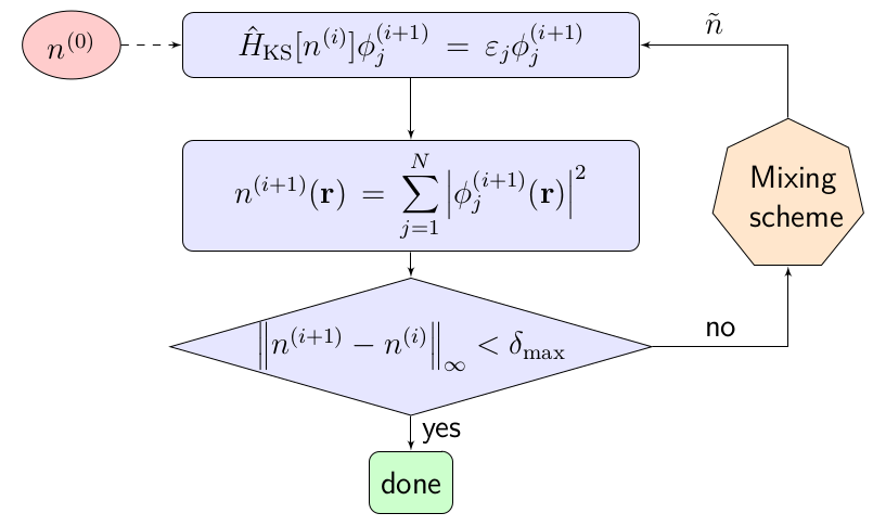
Self-consistent field loop flow diagram.

The SCF loop is an iterative approach which tries to bring the Kohn-Sham equations closer and closer to self-consistency. First, it starts with an initial density $n^{(0)}$ , which is typically chosen to be the sum of the electronic densities associated with the individual atoms. From this starting density we can compute the Hamiltonian $\hat{H}_{\textrm{KS}}[n^{(0)}]$ , and the associated eigenvalue problem can be solved to obtain the eigenenergies $\varepsilon_j$ and eigenstates $\phi_j^{(1)}$ . We assume that we are searching for a ground state, so the $N$ lowest energy eigenstates are filled. By summing the amplitudes squared for these states we get the next electronic density $n^{(1)}$ . This new density is compared to the previous under some distance metric, and if the distance is less than a specified tolerance $\delta_{\textrm{max}}$ , the process is terminated, and if not, the new density is once again used to create an eigenvalue problem. The new density is often modified through a mixing scheme first to help with convergence and to dampen oscillations. A simple class of these methods are linear mixing schemes, where the new trial density is a weighted average of past densities $n^{(i)}$, $n^{(i-1)}$, $n^{(i-2)}$, $\ldots$

To understand why this is usually necessary, consider the phenomenon of “charge sloshing”, as shown below.

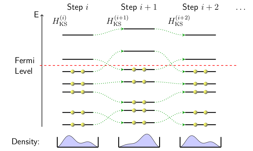
Charge sloshing—an overcompensation while redistributing electronic density from one SCF step to the next.

In the above schematic, $N$ lowest eigenstates (depicted by horizontal lines sorted by energy) corresponding to the Kohn-Sham system at step $i$ in an SCF loop are filled with electrons. These states determine the electronic density of the $(i+1)$ th step, as well as the associated Kohn-Sham Hamiltonian $H_{\textrm{KS}}^{(i+1)}$ , which has its own set of eigenstates. The green dotted lines link the $i$ th states to the $(i+1)$ th states with the most similar character (e.g. as dictated by symmetry, spatial distribution, etc.). The depictions of electrons in a box at the bottom of each step serve to illustrate what the density might look like given the specified filling of the eigenstates.

Notice that the two states straddling the Fermi level “switch positions” from one step to the next. Supposing that one state corresponds to having a higher concentration of charge on the left of the box while the other corresponds to having more charge on the right, the schematic at the bottom shows how the electronic density might be distributed from one step to the next. This is the origin of the term charge sloshing, with electrons moving around from one SCF step to the next much like water in a carried pan. Mixing schemes are used to average the densities of the past SCF states, suppressing the overcompensating charge redistributions.

Without using a mixing scheme, SCF loops rarely converge. In the animation below, an ozone molecule starting with a standard atomic orbital density distribution is run through a few SCF steps. Notice how a minute difference in charge distribution amplifies into an extreme sloshing situation where the majority of the electronic density is placed on the leftmost atom, only to be swapped to the rightmost atoms the very next step.

Charge sloshing on an ozone molecule when no mixing scheme is applied.

Charge sloshing is not always a two step cycle. In more complex systems, it can have a longer period, possibly alternating between a number of configurations equal to a multiple of degeneracies due to symmetry, or sometimes it never settles in to a repeating pattern at all. This final case can be problematic even when mixing schemes are applied. For example, consider the animation below showing the attempted SCF convergence of a ruthenium-55 nanoparticle’s ground state. Even with Pulay mixing applied, an effective standard mixing scheme, the Kohn-Sham system does not reach convergence.

Charge sloshing on a ruthenium-55 nanoparticle. The isosurfaces of density difference on the right show that despite the relatively unchanging electronic energy, the system, the electronic configuration is changing significantly from step to step.

On the left, an inset shows that despite the appearance of a plateau in the energy curve, the system’s electronic energy is still changing from step to step. The energy plotted is relative to the actual ground state of the system, so the depicted states are still more than 0.1 eV away from converging to the lowest energy state. The isosurfaces of the step-to-step difference in density are plotted on the right, with the blue surfaces corresponding to a positive change in electronic density, and the red surfaces corresponding to a negative change. The flashing between blue and red isosurfaces is conveying charge sloshing, this time without a clear periodic pattern in the sequence of SCF steps.

Imaginary-Time Time-Dependent DFT (it-TDDFT)

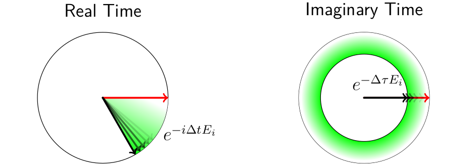
To get around the limitatons of SCF when converging challenging systems, we use a well-known trick in quantum mechanics: imaginary time propagation. This approach exploits the fact that any quantum state is a linear combination of eigenstates of the Hamiltonian, and that by evolving a state in imaginary time the amplitudes of each eigenstate shrink at a rate proportional to the exponential of its eigenenergy. As imaginary time evolution continues, the original state converges to its lowest energy component state, which is usually the ground state.

Imaginary Time Propagation (ITP)

Imaginary time propagation is the formal substitution of $t \rightarrow -i\tau$ wherever time $t$ appears. It is a mathematical trick and not related to an actual physical process, but this transformation often usefully relates physical equations from different domains. To be specific, the central equations of quantum physics and thermal physics happen to be linked by analytic continuation over time, providing a bridge between much of the math in each field. There might be something profound here that physicists have yet to discover, but for our purposes we are just using it as a convenient mathematical tool.

To briefly explain why ITP boosts the lower-energy components of a quantum state, first consider the evolution of an arbitrary state $\ket{\Psi(t=0)} = \sum_{j=0}^{\infty} A_j(t=0) \ket{\Phi_j}$ in terms of eigenstates of the Hamiltonian $\ket{\Phi_j}$ and corresponding eigenenergies $E_j$ :

\begin{equation} \ket{\Psi(t)} = e^{-\frac{it}{\hbar}\hat{H}} \ket{\Psi(0)} = \sum_{i=0}^\infty A_j(t) \ket{\Phi_j} \label{eq:real_time_evolution} \end{equation} \begin{equation} A_j(t) \equiv A_j(0) e^{-\frac{it E_j}{\hbar}}. \end{equation}

The time evolution simply corresponds to a time-dependent rotation of the phase of the amplitudes $A_j(t)$ for each eigenstate in the superposition.

Now, if we apply imaginary time substitution to obtain the equations for imaginary time propagation of the initial state, we get

\begin{equation} \ket{\Psi(\tau)} = e^{-\frac{\tau}{\hbar}\hat{H}} \ket{\Psi(0)} = \sum_{i=0}^\infty \mathcal{A}_j(\tau) \ket{\Phi_j} \label{eq:imaginary_time_evolution} \end{equation} \begin{equation} \mathcal{A}_j(\tau) \equiv \mathcal{A}_j(0) e^{-\frac{\tau E_j}{\hbar}}, \quad \textrm{where} \quad \mathcal{A}_j(0) \equiv A_j(0). \end{equation}

Under imaginary time evolution, the amplitudes $\mathcal{A}_j(\tau)$ tend to shrink as $\tau$ increases, at a rate proportional to the exponential of the energy of the state $E_j$ . The lowest energy state will shink the slowest, and when the unit norm of the state is maintained, i.e. $\Omega(\tau) \equiv \braket{\Psi(\tau) | \Psi(\tau)}$ , $\ket{\tilde{\Psi}(\tau)} \equiv \frac{1}{\sqrt{\Omega(\tau)}} \ket{\Psi(\tau)}$ , the state will eventually purify into its lowest energy component $\ket{\Phi_\ell}$ ,

\begin{equation} \lim_{\tau \to \infty} \ket{\tilde{\Psi}(\tau)} = \ket{\Phi_\ell}, \end{equation}

where $ \ell \equiv \textrm{argmin}_{j} \{E_j\, | \, A_j(0) \neq 0\}$ . Usually, $\ell = 0$ unless the starting state possesses some symmetry or character that is incompatible with the ground state, ensuring that $A_0(0) = 0$ .

To demonstrate what it looks like when ITP “cools” a quantum state into the ground state, the plot below shows the amplitudes $\tilde{\mathcal{A}}_j(\tau) \equiv \frac{\mathcal{A}_j(\tau)}{\sqrt{\Omega(\tau)}}$ of a state composed of four eigenstates as it is propagated in imaginary time.

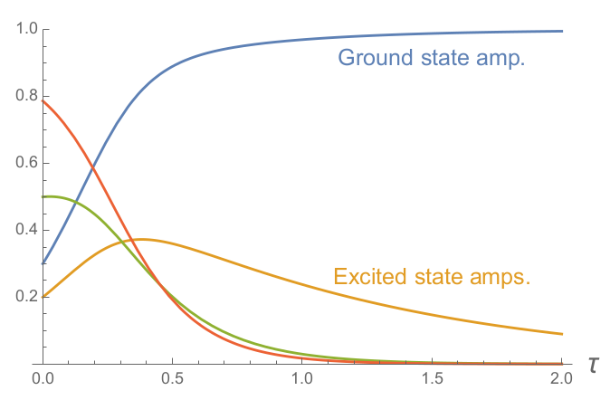
$Cooling an arbitrary quantum state into the ground state component, shown in blue. At $\tau=0$, the initial state is a superposition of four eigenstates. Imaginary time evolution causes lower energy states to become a larger fraction of the superposition until the ground state amplitude eventually dominates.$

Cooling an arbitrary quantum state into the ground state component, shown in blue. At $\tau=0$ , the initial state is a superposition of four eigenstates. Imaginary time evolution causes lower energy states to become a larger fraction of the superposition until the ground state amplitude eventually dominates.

Applying ITP to TDDFT

We can apply the same trick to the time-dependent Kohn-Sham system in order to converge the electronic density to the ground state configuration. This is easily achieved in most TDDFT codes by simply replacing time with imaginary time, promoting the variable to a complex number. The only other constraint is to reestablish the unit norm of the Kohn-Sham wavefunction before taking the next timestep. Despite how straightforward it sounds, there are some nuances to applying imaginary time propagation to TDDFT through the Kohn-Sham system. Remember that the KS system is fictious, and its value lies in its mathematical link to the density of the real system. It is not obvious that ITP of KS system produces a density that emulates ITP of the real system. However, it turns out that imaginary time evolution of the real system through the KS system is justified, as shown through an extension of the van Leeuwen theorem proven in my paper. This connection also justifies the use of imaginary-time methods in TDDFT in a physically meaningful way, like in this accurate treatment of ionic zero-point motion in DFT presented by my co-authors. We chose to refer to imaginary-time time-dependent density functional theory as it-TDDFT.

Returning to the ozone example, the animation below shows how it-TDDFT is a much more stable method than unmixed SCF. Even when starting with all the electrons on one side of the molecule, it-TDDFT is easily able to converge the system to its ground state.

Imaginary-time TDDFT is a robust way to converge an electronic system to its ground state, even when starting from a bad configuration.

In the figure below, we applied it-TDDFT to find the ground state of a benzene molecule. The plotted isosurfaces are showing the density difference to the ground state (as obtained by SCF) at various points in the trajectory through imaginary time. The isosurfaces shrink as the density difference approaches zero, meaning that the method has found the ground state. The system’s electronic energy, plotted in black, is also measured relative to the ground state energy. Finally, the blue curve shows the value of half the $L^1$ distance between the instantaneous density and the ground state density, which has the natural interpretation of “the number of electrons out of place” relative to the reference ground state density.

Using it-TDDFT to find the ground state of a benzene molecule. Isosurfaces of the density difference to the ground state are shown, and $D[n,n_0]$ is half the $L^1$ distance between the instantaneous density and the ground state density.

Notice that the electronic energy decreases monotonically, and that the density smoothly approaches the ground state. It is also interesting to note that the “electrons out of place”, as measured by the blue curve, plateaus for a while even as the energy continues to decrease. This is possible since the electronic density that is not overlapping with the ground state density can be rearranged to continue decreasing the energy.

For a more challenging example, we also applied it-TDDFT to the ruthenium-55 nanoparticle that SCF had trouble with. In contrast to the earlier animation, this system poses no issue for imaginary time propagation, and the ground state is readily found.

Using it-TDDFT to find the ground state of a ruthenium-55 nanoparticle. Isosurfaces of the density difference to the ground state are shown, and $D[n,n_0]$ is half the $L^1$ distance between the instantaneous density and the ground state density. This system was very challenging to converge with SCF and Pulay mixing due to charge sloshing issues, but imaginary time propagation progresses towards the ground state with ease.

Finding Excited States

The it-TDDFT approach can also be used to find excited states, much in the same way as when applying ITP to find excited states in single-particle quantum mechanics. However, it is challenging to maintain orthogonality of higher energy eigenstates to the states that have already been found due to the fact that orthogonality of states in the KS system is not necessarily equivalent to orthogonality of states in the real physical system. An easy way to see this is by remembering that in the KS system, the Hamiltonian is a functional of density. Since the density changes with each excited state, ensuring orthogonality of the highest occupied KS orbital to unoccupied orthogonal orbitals below it does not have a clear connection to orthogonality considerations in the real system. That said, the naive approach of retaining unoccupied KS orbitals below the highest occupied orbital can still serve as an approximation, especially when the low-lying excited state densities of a system are not very different from the states below them. Additionally, this is already the standard approach used to find excited states with SCF, called Delta SCF, so this approach remains consistent with the standard methods in the field. Finding a way to generally apply it-TDDFT to find excited states could be an avenue for future research.

In the animation below, we compute the approximate first four excited states of a helium atom using it-TDDFT and the naive KS orbital orthogonality approach where we propagate unoccupied orbitals alongside the occupied ones in imaginary time. This results in excited states that are equivalent to what would be found with standard Delta SCF. Notice how the method finds the $2s$ , $2p_x$ , $2p_y$ , and $2p_z$ excited states.