Neural Network Solution Bundles
Jun 17, 2020 | 7 min read | technical
Many dynamical systems are described by ordinary differential equations (ODEs) which relate the rates and values of quantities to describe how they evolve in time. While some simple ODEs have closed-form solutions, like the exponential function for radioactive decay, sines and cosines for harmonic oscillators, and the logistic function for population growth, the vast majority have to be solved approximately using numerical techniques.
Most of these methods seek to numerically integrate the ODEs by starting from initial conditions and stepping forward until the desired final time is attained. This means that if we want to know the state of a system at some later time, we first have to compute a sequence of states at earlier times, which is inefficient if these intermediate states are not used for other purposes. In addition, we are typically interested in a family of solutions to the ODE for different initial conditions and parameters. Ideally, we would want a function that outputs a system’s state given initial conditions, parameters, and a time.
Neural networks are great candidates for this task since they can represent arbitrary functions, and through an appropriately chosen loss function the neural net can learn a bundle of solutions to the ODEs without any reliance on data computed by conventional methods.
Learning a Bundle of Solutions
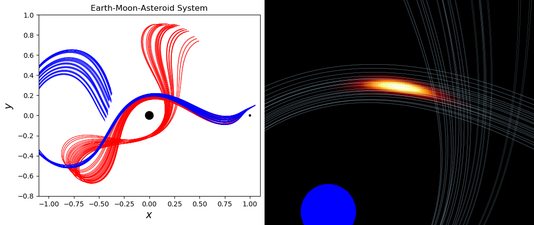
The above video shows the training of a neural network solution bundle for the planar circular restricted three-body problem, e.g. the orbit of an asteroid in the plane of the co-orbiting Earth and Moon. In red, trajectories for asteroids with different inital conditions (initial positions and velocities) are plotted, computed with Runge-Kutta, a conventional method for solving ODEs. In blue we show the corresponding trajectories in the neural network solution bundle, which converge towards the true trajectories as the network is trained.
This training method is unsupervised, so the neural network is given no knowledge of the trajectories in red. It only seeks to best satisfy the differential equations that govern this system.
Using a Neural Network Solution Bundle
Once we have the bundle of solutions, computing the state of the system at any time or initial condition encompassed by the training set takes $\mathcal{O}(1)$ time. This makes it computationally cheap to evaluate a variety of configurations at a variety of times, which is convenient when we wish to consider a distribution of system states simultaneously.
Propagating a Distribution
$\mathbf{x}_0$ described by a 2D normal distribution, and we show its position at later times. The distribution of its positions $\mathbf{x}(t\,;\,\mathbf{x}_0 )$ at time $t$ can be calculated directly by iterating over the initial conditions and weighting by the corresponding probability densities. While a similar calculation can be done with standard stepping methods like RK4, the benefit of the solution bundle approach is that we can calculate the distribution of states at time $t$ directly, without having to compute the intermediate states at earlier times.
Bayesian Inference
Another situation where fast evaluations of many different system configurations can be helpful is for Bayesian inference, where we wish to estimate the parameters governing a differential equation based on observed data. When computing the distributions of a dynamical system’s parameters using, solutions associated with each set of potential system parameters have to be evaluated at every time corresponding to a data point. Since a neural network solution bundle for the system can calculate the state at any time and configuration of parameters in the same amount of computational time, the contribution of every data point along the trajectory can be efficiently computed in parallel.
Example: Rebound Pendulum
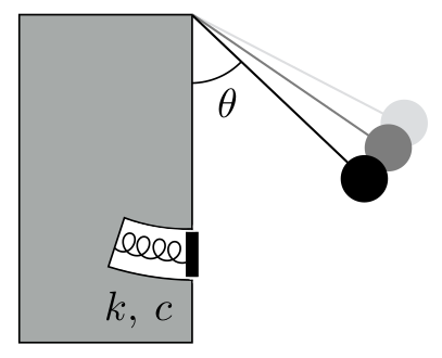
Diagram of a rebound pendulum.
A rebound pendulum consists of a simple pendulum that can collide with a damped spring at the bottom of its swing. This system approximates a standard test method for rubber resilience used in the materials industry, where the pendulum hammer impacts a material sample and its energy dissipation, impact time, and maxmimum indentation depth can be used to infer various properties of the sample. In the above diagram, $k$ is the spring constant, and $c$ is the damping coefficient.
First, we train the neural network solution bundle for the initial condition and parameter range we are interested in. The following image shows a few trajectory samples from the solution bundle, and the NN solution bundle samples are shown in blue, while reference RK4 trajectories are underlayed in red.
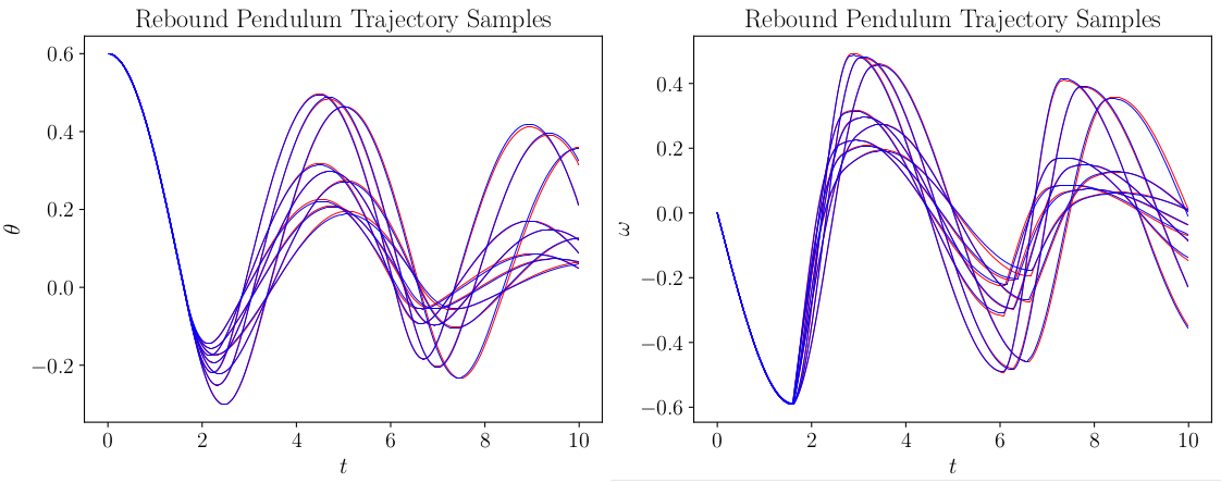
A few trajectories from the neural network solution bundle for a rebound pendulum.
Suppose we have measured the following data points in yellow and we want to estimate the most likely initial conditions $(\theta_0,\omega_0)$ and system parameters $k, c$ given the data. Using Bayesian inference, we can estimate these quantities as shown below.
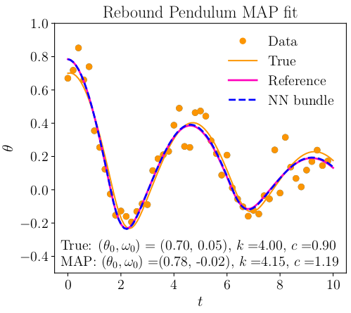
Maximum a posteriori fit for the rebound pendulum data.
The true trajectory using the exact system parameters is shown in yellow, and the NN bundle Bayesian estimate is shown in blue, overlayed on a reference RK4 trajectory with the same parameters to confirm its accuracy.
Bayesian inference separates itself from a simple least-squares fit by also providing estimates of the uncertainty of the estimated parameters through the marginal posterior distributions, shown below.
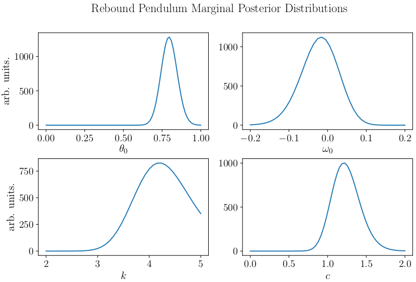
Marginal posterior distributions for the initial conditions and parameters of the system.
How it Works
Neural network solution bundles are an extension of the Lagaris method (arXiv) for unsupervised training of neural networks to solve ODEs and PDEs for a single set of initial/boundary conditions. We have expanded the method to produce solution bundles across a set of initial conditions and parameters.
Consider the following general first-order differential equation parameterized by $\boldsymbol{\theta}$:
$$ \mathbf{G} \left( \mathbf{x}, \frac{\textrm{d} \mathbf{x}}{\textrm{d} t}, t \,;\, \boldsymbol{\theta} \right) = 0, $$
where $\mathbf{x} \in \mathbb{R}^n$ is a vector of state variables, $t$ is time, and $\boldsymbol{\theta} \in \mathbb{R}^p$ are physical parameters associated with the dynamics. The solutions to the differential equation over the time range $[t_0, t_f]$, together with a subset of initial conditions $X_0 \subset \mathbb{R}^n$ and a set of parameters $\Theta \subset \mathbb{R}^p$ define a solution bundle $\mathbf{x}(t\,;\, \mathbf{x}_0, \boldsymbol{\theta})$, where $\mathbf{x}_0 \in X_0$, $\boldsymbol{\theta} \in \Theta$.
We create an approximating function for the solution bundle over $(X_0, \Theta)$ using the form
$$ \hat{\mathbf{x}}(t \, ; \, \mathbf{x}_0, \boldsymbol{\theta}) = \mathbf{x}_0 + a(t) \mathbf{N}(t \, ;\, \mathbf{x}_0, \boldsymbol{\theta} \, ;\, \mathbf{w}),$$
where $\mathbf{N}: \mathbb{R}^{1+n+p} \rightarrow \mathbb{R}^n$ is a neural network with weights $\mathbf{w}$, and $a : [t_0, t_f] \rightarrow \mathbb{R}$ satisfies $a(t_0) = 0$. This form explicitly constrains the trial solution to satisfy the initial condition $\mathbf{x}(t_0) = \mathbf{x}_0$.
The training is performed with an unsupervised loss function,
$B = \left\{(t_i, \mathbf{x}_{0i}, \boldsymbol{\theta}_i)\right\}$ constitutes a training batch of size $|B|$, with $t_i \in [t_0, t_f]$, $\mathbf{x}_{0i} \in X_0$, and $\boldsymbol{\theta}_i \in \Theta$ drawn from some distribution over their respective spaces. The function $b: [t_0,t_f] \rightarrow \mathbb{R}$ in the loss function is used to weight data points based on their time, and it can help with convergence and balancing the absolute error across the trajectory.
The intuition behind the loss function is that the network is essentially performing “guess and check” on the differential equation. For each time, initial condition, and set of parameters within the training batch, the left side of the differential equation $\mathbf{G} \left( \hat{\mathbf{x}}, \frac{\partial \hat{\mathbf{x}}}{\partial t}, t \,;\, \boldsymbol{\theta} \right)$ is evaluated exactly, and the goal is to bring these values as close to zero as possible. Since $\mathbf{G}$ evaluates to zero for solutions to the differential equation by definition, the loss function is chosen to have a minimum value of zero, achievable when the NN solution bundle exactly matches the local behavior of a solution at every point in the batch. With each batch randomly sampled across the training region, eventually the NN solution bundle approximates the true solution bundle as well as it can.
For additional technical information and examples, check out our submission on arXiv.