Outguessing a Riffle Shuffle
Jun 24, 2026 | 18 min read | technical
How many riffle shuffles does it take before a freshly-ordered deck becomes genuinely unpredictable? The folklore answer is “seven.” I trained a small transformer to guess the next card after $k$ shuffles (handing it the deck’s starting order and letting it watch every card as it was dealt), and it kept finding a usable edge well past seven, all the way out to eleven.

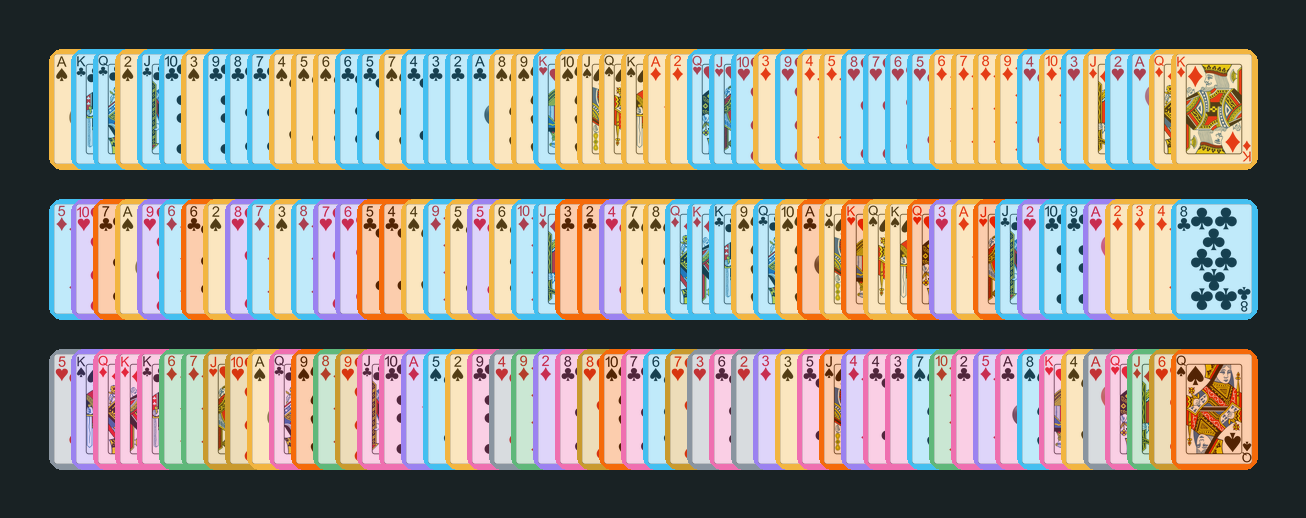
Each card tinted by the packet it came from. Top: after one riffle the deck is just two interleaved runs. Middle and bottom: two shuffles leave up to four. Those bands of color are exactly the structure a predictor learns to exploit.
I play a lot of board games, card games, and Magic: The Gathering, and the humble shuffle has always appealed to me. In any game with a deck, the shuffle is where so much of the interesting stuff comes from: it’s the built-in bit of chaos that everyone at the table has to read and plan around. It also tends to provoke a small ritual argument, because there’s always someone who insists the cards are plenty shuffled already and we should just deal. The folklore on their side has a famous number attached to it: seven shuffles is enough to randomize a deck of cards, a claim that traces back to a 1990 New York Times article about Bayer and Diaconis’s work. I wanted to poke at it from a slightly different angle than usual. Instead of measuring how far a shuffled deck sits from random, I asked a more operational question: can a neural network actually predict the next card? It’s a concrete handle on the same idea, since any structure a predictor can exploit is structure the deck hasn’t yet shuffled away.
The setup is simple to state. We start from a deck in a known order, shuffle it some number of times, and then deal it out one card at a time. At each step the predictor has already seen every card dealt so far, and it tries to name the next one. How well it can do that, as a function of how many times we shuffled, is the whole story.
Why a shuffled deck is predictable at all
A riffle shuffle is far less random than it looks. You cut the deck into two packets and interleave them, but crucially you never reorder the cards within a packet. So immediately after one shuffle, the deck is nothing more than two ascending runs woven together.
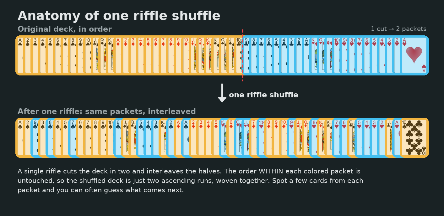
Anatomy of a single riffle. The deck is cut into a top packet and a bottom packet, then interleaved. Within each packet the original order is perfectly preserved.
Once a few cards have come out, those two packets become obvious, and the next card has to be the head of one packet or the other: just two candidates instead of fifty-two. If you always bet on the head of the larger remaining packet, you are right more than half the time. Compare that to the couple of percent you would expect from a blind guess.
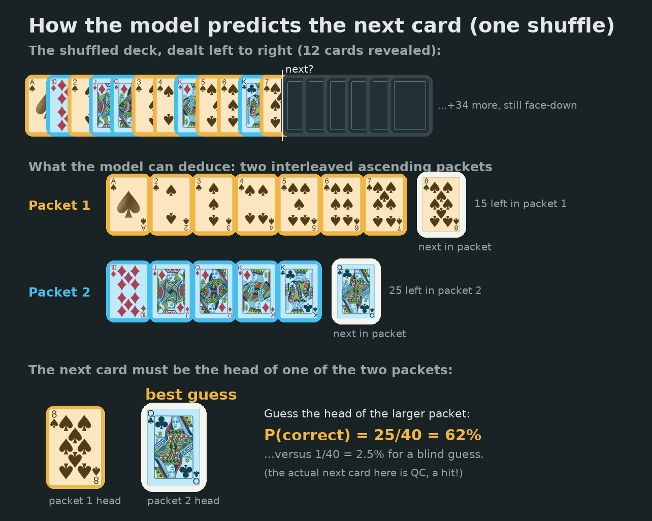
After one shuffle the next card is always the head of the top packet or the head of the bottom packet. Betting on the longer packet wins the majority of the time.
Every additional riffle roughly doubles the number of interleaved packets: two shuffles give up to four, and $k$ shuffles give up to $2^k$. More packets mean more candidates for the next card, so the predictable edge should shrink geometrically as the shuffles pile up. That intuition turns out to be exactly right, and watching it play out quantitatively is most of the fun.
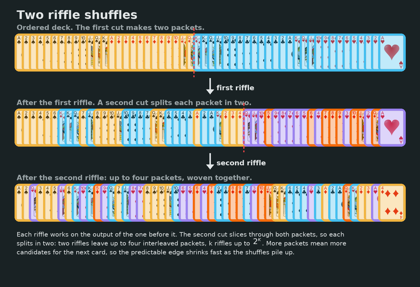
Two shuffles. The clean two-packet picture fractures into as many as four interleaved runs, and the predictable structure starts to wash out.
So the whole experiment is really this: train a network to spot the packets and bet on the most likely next card, then measure how much of that structure survives each successive shuffle.
What the model sees
Each training example is a single sequence of 107 tokens, drawn from a vocabulary of 56 (the 52 cards plus four special tokens for start, separator, mask, and end), laid out like this:
[ ^ | original deck order (52) | separator | dealt cards (52) | $ ]
The model is a small 2-layer, 2-head Transformer encoder (embedding dimension 128, feed-forward dimension 256, about 293k parameters) with learned absolute positional embeddings, which I’ll call TransformerModel(128, 256). It trains with a causal, language-model-style objective: a single triangular attention mask means the prediction for each of the 52 dealt cards is conditioned on the entire original deck order plus every earlier dealt card. Because the full starting deck sits in front of the dealt cards, one forward pass scores all 52 dealt positions at once, roughly 52× more signal per step than predicting a single position. Everything ran on CPU (no GPU), 1M iterations per model, about 35 hours of wall-clock each (graciously absorbed by some free cloud compute that I felt no guilt whatsoever about fully utilizing).
Two assumptions are baked in, and both matter when you read the numbers:
1. The starting order is known. This is unavoidable rather than a modeling shortcut. If the deck began in an unknown, uniformly random order, the next card would be uniformly random no matter what had been dealt, and there would be nothing to predict. So I always start from the canonical sorted order. This loses no generality: any known starting order is equivalent by symmetry to the sorted one. You relabel the cards so the known start becomes canonical, run the model, then map the prediction back through the same relabeling. Collapsing that symmetry lets a fixed-order model spend all of its capacity on the part that actually varies: the shuffle.
2. Complete feedback. The model sees every previously dealt card when it predicts the next one. This is the standard “card guessing with complete feedback” setting, and it is what ties the one-shuffle result to a known optimal strategy below. The harder no-feedback variant is a genuinely different problem.
I evaluated each of the eleven trained models (one per shuffle count, $k = 1$ through $11$) with 10 million samples per dealt position, about 520M predictions per model. That brings the 95% confidence intervals down to roughly $\pm 0.003\%$, which matters a lot once we are out hunting for tiny effects near the tail.
What the network learned
Here is the headline plot: per-position prediction accuracy against the number of cards already dealt, one curve per shuffle count, with the dashed line showing the random baseline $1/R$ where $R$ is the number of cards still face down.
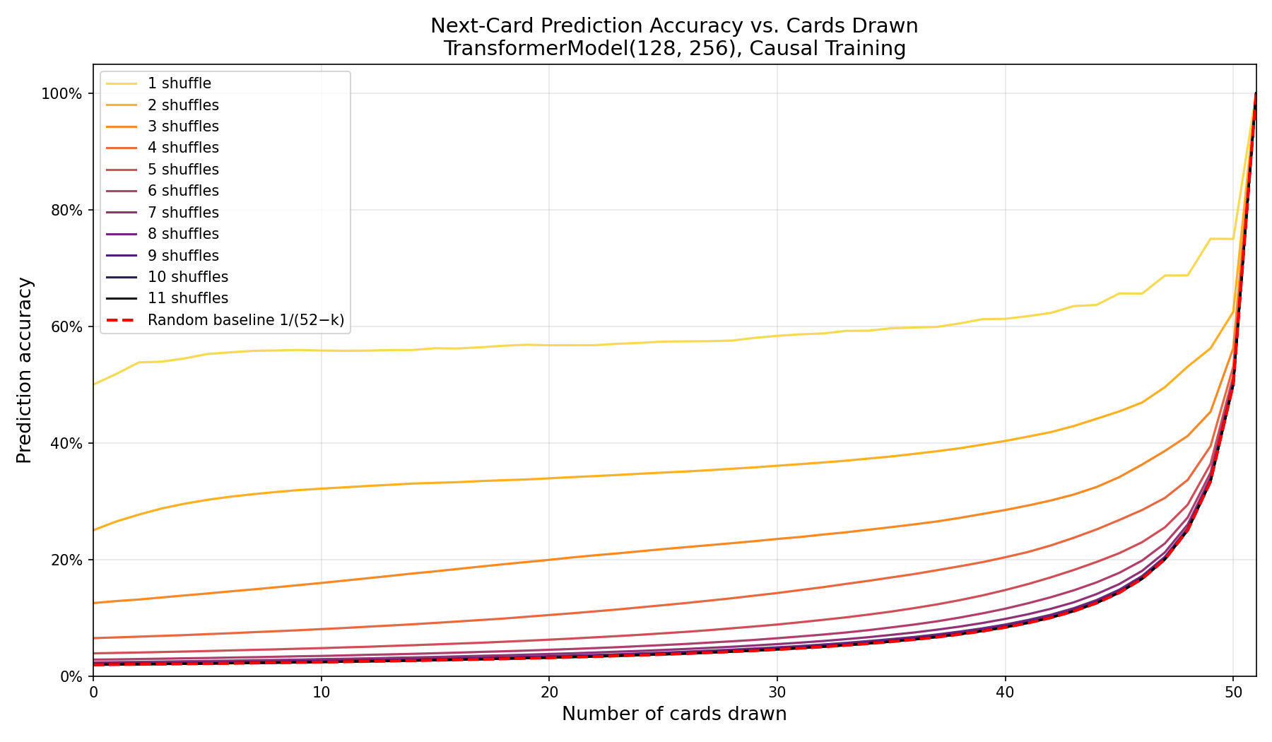
Next-card accuracy versus cards drawn. One shuffle (top curve) starts at 50% from the very first card and climbs toward 100% as the deck empties out; each additional shuffle peels another curve down toward the random baseline.
One shuffle is wildly predictable: even the very first card can be named correctly half the time, and accuracy only climbs from there as the dealt cards constrain what’s left. The first-card figure is the surprising one, and it tripped up my own intuition at first. You’d think you would need to know where the deck was cut to guess it, and you don’t. The card that started on top stays at the top of its packet no matter where the cut falls, so it leads the deal whenever the first card comes off that packet, which by symmetry happens half the time. Guessing “the card that started on top” is therefore right about 50% of the time. The card you genuinely can’t call is the one just below the cut, the head of the bottom packet, because the cut location is random and smears its likelihood across all the cards near the middle of the deck. Each extra shuffle drops the next curve sharply toward the baseline. By eye, somewhere around six or seven shuffles the curves start to pile up near random and become hard to tell apart. We will need a better lens for the tail, but first I want to dwell on the one-shuffle curve, because it hides a lovely little sanity check.
The one-shuffle curve knows its combinatorics
The one-shuffle curve has fine structure at both ends, and each end is a fingerprint of the optimal Bayesian strategy. They turn out to be mirror images of each other. The head of the curve, the first cards off the deck, is the model still inferring where the deck was cut. The tail, the last few cards, is the model knowing the cut exactly and sweating the parity. Let’s take them in turn.
We just saw that the first card is a coin flip, because the cut is the one thing the model can’t see. Here is what happens as the cards start coming out. The random baseline this early is only about 2%, so every number below is better than a 25x lift over chance:
| Cards dealt | Accuracy |
|---|---|
| 0 | 50.00% |
| 1 | 51.81% |
| 2 | 53.81% |
| 3 | 53.93% |
| 4 | 54.49% |
| 5 | 55.24% |
| 6 | 55.53% |
| 7 | 55.79% |
| 8 | 55.85% |
| 9 | 55.93% |
| 10 | 55.84% |
| 11 | 55.80% |
| 12 | 55.82% |
| 13 | 55.91% |
Accuracy climbs about six points over the first eight cards, and the cause is exactly the cut. Every dealt card sharpens the model’s estimate of where the deck was split, so its best guess gets a little better each time. It starts at $26/52 = 1/2$ (the expected cut sits dead center) and rises as the estimate tightens. The instant cards from both packets have appeared, the gap between the two ascending runs pins the cut down exactly, and from there the “bet on the bigger packet” logic of the tail takes over.
The fun part is that the climb is genuinely jagged, not a smooth ramp, and it isn’t noise: the per-point error bars are about $\pm 0.03\%$. The steps are wildly uneven, +2.0 points from the 2nd card to the 3rd but only +0.12 from the 3rd to the 4th, and there’s even a real little local peak at 9 cards dealt (55.93%) followed by a two-card dip before the climb resumes. These are the head-of-deck counterpart to the tail ripples below: the cut is a whole number, the model’s belief about it is a discrete distribution, and the same parity and combinatorial corners that wrinkle the tail show up here while the split is still being resolved.
Now the other end. Zoom in on the tail of the one-shuffle curve and you’ll see small but unmistakable “ripples.” Accuracy doesn’t fall smoothly as the deck empties; it comes in roughly flat pairs:
| Cards remaining | Accuracy |
|---|---|
| 7 | 65.64% |
| 6 | 65.61% |
| 5 | 68.70% |
| 4 | 68.73% |
| 3 | 75.01% |
| 2 | 75.00% |
| 1 | 100.00% |
These ripples are real, not noise, and they are a fingerprint of the single shuffle’s combinatorics. After one riffle, the deck is the interleaving of a top packet of size $T \sim \mathrm{Binomial}(52, \tfrac{1}{2})$ and a bottom packet of size $52 - T$. The model can always match each dealt card to its packet of origin, so at every step it knows exactly how many cards remain in each, call them $T_{\text{rem}}$ and $B_{\text{rem}}$, with $T_{\text{rem}} + B_{\text{rem}} = R$.
The optimal predictor bets on the head of whichever packet is longer, so its accuracy is about
$$ \mathbb{E}\!\left[\frac{\max(T_{\text{rem}},\, B_{\text{rem}})}{R}\right]. $$Now parity matters. When $R$ is even, the worst case $T_{\text{rem}} = B_{\text{rem}} = R/2$ is possible, and at that draw you are reduced to a 50/50 coin flip. When $R$ is odd, the split is forced to be unequal, so that dead zone is impossible. That is precisely the pattern in the table: each odd-$R$ draw clusters with the next-smaller even-$R$ draw at slightly higher accuracy, because the odd draws can never fall into the 50/50 trap. The wiggles grow toward the tail because the distribution over splits concentrates on small integers there, where the parity effect is largest.
For two or more shuffles the clean two-packet structure is gone, the conditional distributions smooth out, and both the jagged head and the rippled tail vanish. The fact that they show up only for one shuffle, sharp combinatorial corners and all, is a delightful sign that the network didn’t just learn a fuzzy heuristic. It reconstructed the optimal Bayesian strategy almost perfectly, at both ends of the deck.
And we can check the size of that edge against theory. For one riffle shuffle with complete feedback, Liu (2021) proved that the optimal rule is exactly this “two packets, bet on the head of the longer one” strategy (with $\Pr(\text{next} = \text{head of } A) = |A| / (|A| + |B|)$), and that the expected number of correct guesses it earns is
This is an asymptotic result: the two leading terms are what the reward converges to as the deck grows, but for any finite deck there’s a bounded correction the proof leaves unspecified. Liu notes the technique can’t pin down its value, only that it stays small. For $n = 52$ the leading terms alone come to $31.75$ cards, about 61%, and if you take that as the target then our 59.665% looks like it’s leaving more than a full point on the table.
It isn’t. The optimal strategy is known exactly even when its closed-form reward isn’t, so you can just compute what that strategy actually scores on 52 cards instead of trusting the asymptotic. That number is exact rather than simulated: a short recursion over the optimal play, cross-checked against brute-force optimal play on small decks, puts the true optimum at 59.94% (about 31.17 cards), not 61%. The asymptotic formula overshoots a real deck by a little over half a card, which is the whole of that missing $O(1)$. The paper only states the asymptotic, so this exact 52-card figure isn’t written down there, even though it falls right out of their strategy.
Against that target, our model’s 59.665% is about a quarter of a percentage point short of optimal. It isn’t playing perfectly: the gap is real rather than noise, sitting far outside our $\pm 0.003\%$ error bars.
Watching the edge decay
The absolute-accuracy plot squashes all the high-shuffle curves together, so to see the tail I divided each model’s accuracy by the random baseline at every position and put it on a log scale. A ratio of 1 means “no better than guessing.”
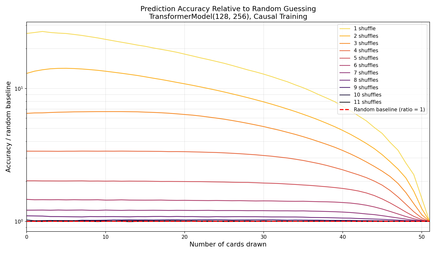
Accuracy divided by the random baseline, log scale. On this view the shuffle counts separate cleanly, and even seven shuffles holds a ratio clearly above 1 across most of the deck.
On this scale the separation is unambiguous, and the low-shuffle curves dominate. Restricting to seven-and-up and refocusing the y-axis lets the residual signal at the very top of the range show itself:
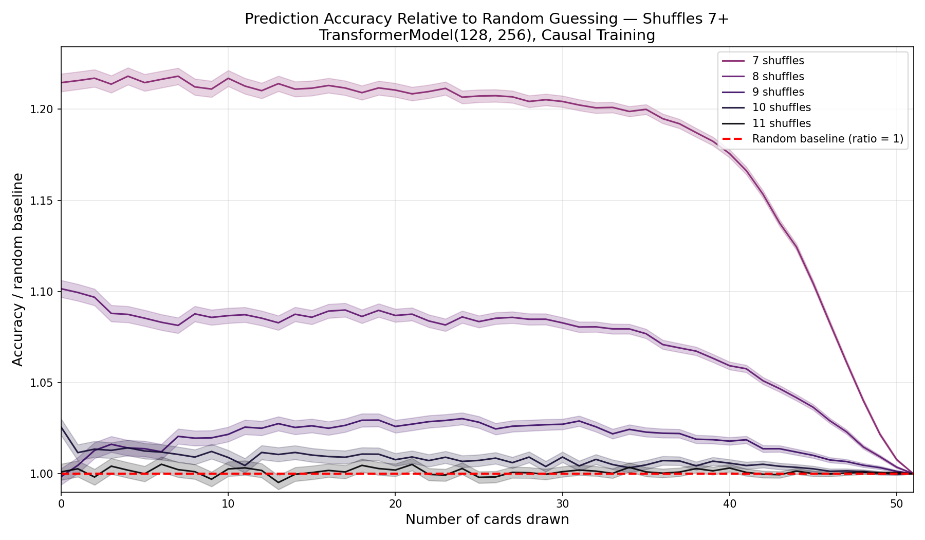
Just the seven-or-more curves, rescaled. Even eleven shuffles sits visibly above the baseline ratio of 1, though only barely.
Even eleven shuffles is detectably above random. Here is the full table of overall accuracies, with confidence intervals and the lift over the 8.727% random baseline:
| Shuffles | Overall accuracy | 95% CI | Lift vs. random |
|---|---|---|---|
| 1 | 59.665% | [59.660%, 59.669%] | +50.94 pp |
| 2 | 37.919% | [37.915%, 37.923%] | +29.19 pp |
| 3 | 24.829% | [24.826%, 24.833%] | +16.10 pp |
| 4 | 16.811% | [16.808%, 16.814%] | +8.08 pp |
| 5 | 12.525% | [12.522%, 12.528%] | +3.80 pp |
| 6 | 10.515% | [10.512%, 10.518%] | +1.79 pp |
| 7 | 9.557% | [9.554%, 9.559%] | +0.830 pp |
| 8 | 9.046% | [9.043%, 9.048%] | +0.319 pp |
| 9 | 8.819% | [8.817%, 8.822%] | +0.092 pp |
| 10 | 8.756% | [8.754%, 8.759%] | +0.029 pp |
| 11 | 8.732% | [8.730%, 8.735%] | +0.005 pp |
| Random | 8.727% | n/a | n/a |
A few things jump out:
- One shuffle is barely a shuffle: 50% accuracy from the very first card, climbing toward 60% overall.
- Each extra shuffle attenuates the edge by a roughly geometric factor, but within this range the structure never fully disappears.
- Even eleven shuffles shows a (barely) detectable signal. That +0.005 pp lift is about four standard deviations above zero given our
$\pm 0.003\%$intervals, statistically significant ($p < 0.0001$), but right at the edge of what 10M samples per position can resolve. Pushing to twelve or more shuffles would need dramatically more samples. - The confidence intervals never overlap: each shuffle count is cleanly separated from its neighbors at every position.
I’ll resist over-interpreting that the lift “runs out” at eleven. It doesn’t reach zero at eleven; eleven is just where my sample budget stops being able to see it. With more samples the detectable edge would creep further out.
A note on training
All eleven models trained for 1M iterations with the causal objective, and every one of them plateaued almost embarrassingly early, most within the first 100k iterations.
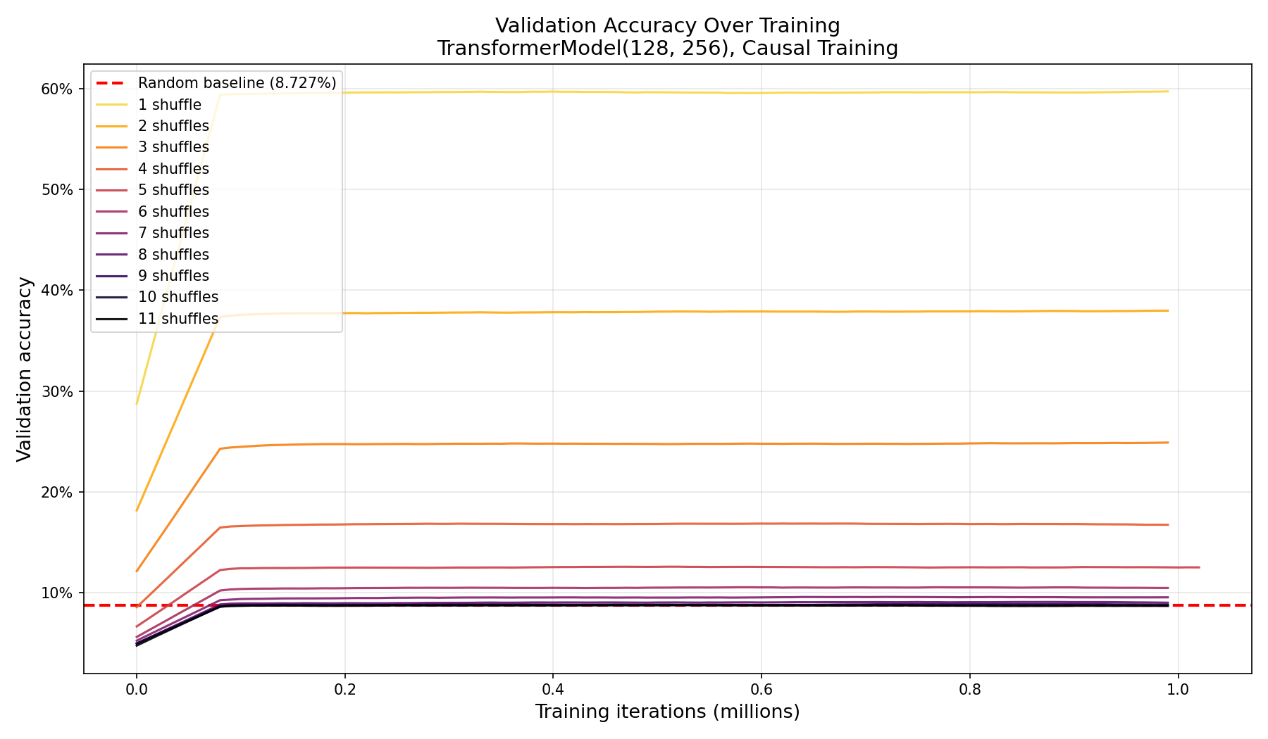
Validation accuracy over training. Each model snaps to its final plateau almost immediately, then holds.
That near-vertical “elbow” looked suspicious, so I plotted the raw, unsmoothed validation accuracy zoomed into the first 250k iterations to rule out a smoothing artifact:
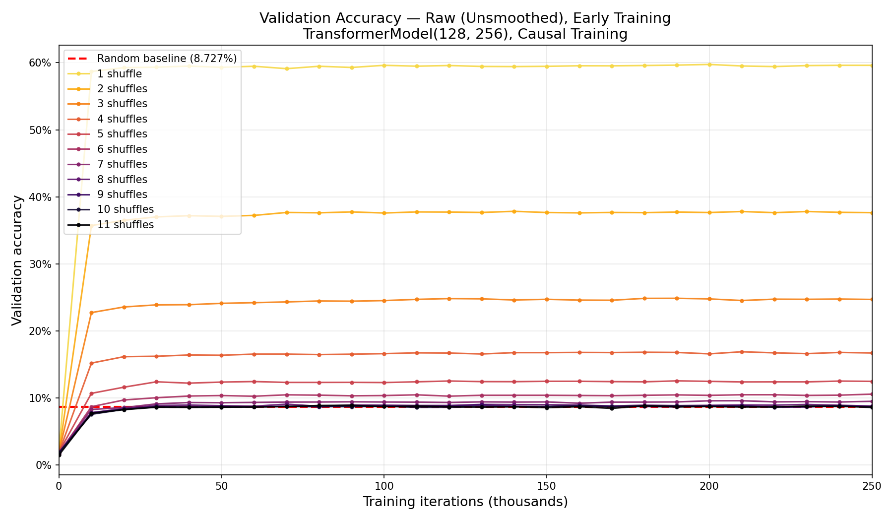
Raw (unsmoothed) early-training accuracy. The elbow is real: the transition just happens between iteration 0 and 10k, faster than the 10k-iteration validation cadence can resolve.
The elbow is genuine; the whole transition happens somewhere between iteration 0 and 10k, faster than my validation cadence could catch. By the first recorded data point, every model is essentially done. With 293k parameters (well above the capacity needed for this task), a causal objective that turns each step into 52 position-predictions, and a tiny 56-token vocabulary, the optimizer reaches near-optimal performance in a few thousand steps and then just sits there.
So, what about “seven shuffles”?
It is worth being precise about what the “seven shuffles” result actually proves. The claim is almost always heard as “the deck becomes uniformly random after seven riffles.” That is not what the theorem says.
The actual result, from Bayer and Diaconis (1992), is about the total variation distance (TVD) between the post-shuffle distribution and uniform. The sharp “cutoff” actually sits at $\tfrac{3}{2}\log_2 n \approx 8.55$ shuffles for $n = 52$ (not seven), building on the strong-uniform-time machinery of Aldous and Diaconis (1986). Their Table 1 gives the TVD at each $k$:
| k shuffles | 1 | 2 | 3 | 4 | 5 | 6 | 7 | 8 | 9 | 10 |
|---|---|---|---|---|---|---|---|---|---|---|
| TVD | 1.000 | 1.000 | 1.000 | 1.000 | 0.924 | 0.614 | 0.334 | 0.167 | 0.085 | 0.043 |
At seven shuffles the TVD is still 0.334, a long way from zero. “Seven” was Diaconis’s practical casino/bridge threshold, the point past which most macroscopic statistics look random, not a claim of true uniformity. My seven-shuffle model hits 9.557% versus the 8.727% baseline, a lift of about 0.83 pp, or a ratio near $1.095\times$. That is exactly the kind of small-but-real signal a residual TVD of 0.334 leaves on the table.
Put together, this says that seven riffles really does make a deck practically random, in the sense that you can’t tell hands apart by eye, while still leaving a sufficiently capable predictor with full information enough structure to pull out about one bit of advantage spread across several dozen cards. The popular version of the result captures something genuinely true about everyday play, even if the stronger reading of it, that the deck has become uniformly random, isn’t quite right.
Some broader context
Once you frame “predict the next card” as the central question, it connects to a surprisingly deep literature.
“Seven” depends entirely on how you measure. Swap TVD for Shannon entropy and you get a different answer: Trefethen and Trefethen (2000) found roughly five to six shuffles, with no cutoff at all: the non-randomness decays smoothly from the first shuffle. They framed it as “the magnitude of a trend versus its statistical significance.” My predictability lift is a magnitude-type quantity, which is exactly why it declines smoothly rather than cliff-edging. As another data point, the stricter worst-case separation distance mixes at $2\log_2 n \approx 11$ shuffles for 52 cards, suggestively close to where my detectable signal runs out, though I want to be clear that’s a numerical echo, not a proven mechanism.
Real shuffles are messier, and mix slower. The model here uses idealized, evenly-split cuts. Real human riffles drop cards in clumps, and clumpiness slows mixing: Jonasson and Morris (2015) proved clumpy shuffles mix in $O(\log^4 n)$, far slower than the idealized $\tfrac{3}{2}\log_2 n$. A recent result (Sellke, Shi, and Wang), popularized by Quanta in 2026, shows that with realistic varied cuts the bar rises to roughly fourteen shuffles, about double the classic seven.
And yes, casinos care. Diaconis, Fulman, and Holmes (2013) analyzed an automatic shelf-shuffling machine and found that one pass left enough structure for a knowledgeable player to guess about 9 to 9.5 of 52 cards correctly, versus about 4.5 for a well-shuffled deck. Diaconis reportedly said it would “double or triple the advantage of the ordinary card counter,” and the manufacturer redesigned the machine.
If you want to go deeper, the standard reference is Diaconis and Fulman’s The Mathematics of Shuffling Cards (AMS, 2023), and the foundational paper is still Bayer and Diaconis (1992), “Trailing the Dovetail Shuffle to its Lair.”
Shuffling up
What started as curiosity about whether a transformer could learn the basic structure left in shuffled cards sent me down a rabbit hole, as the prototype models kept impressing me. I did not expect to push the predictor all the way to the fabled limit of seven riffle shuffles, let alone past it, and I picked up a good deal of the deep theory of shuffling along the way. The headline result still pleases me: a 293k-parameter network, handed a deck’s starting order and complete feedback, plays the one-shuffle game within a quarter-point of provably optimal play (combinatorial parity ripples and all), and keeps finding a small but real edge all the way out to eleven shuffles. The broader lesson is one the mixing-time literature has been making for decades: “random enough” is not a single number, but depends on what you measure and how hard you are willing to look.
So the next time a fellow board gamer waves off the deck as shuffled enough and reaches to deal, we should probably just let them, as it really should be random enough. But maybe let’s just shuffle a few more times, just in case… and maybe a few more times…